Tutorial¶

The Climate Data Operators (CDO) software is a collection of many operators for standard processing of climate and forecast model data. The operators include simple statistical and arithmetic functions, data selection and subsampling tools, and spatial interpolation. CDO was developed to have the same set of processing functions for GRIB and NetCDF datasets in one package.

The Climate Data Interface [CDI] is used for the fast and file format independent access to GRIB and NetCDF datasets. The local MPI-MET data formats SERVICE, EXTRA and IEG are also supported.

There are some limitations for GRIB and NetCDF datasets.
A GRIB dataset has to be consistent, similar to NetCDF. That means all time steps need to have the same variables, and within a time step each variable may occur only once.
NetCDF datasets are only supported for the classic data model and arrays up to 4 dimensions. These dimensions should only be used by the horizontal and vertical grid and the time. The NetCDF attributes should follow the GDT, COARDS or CF Conventions.

Introduction¶

To display all command line options of cdo, type

cdo -h

and to get an overview of all operators with a short description, type

cdo --operators

To get more information about an operator

cdo -h <operator>

The best way to get full information about the operators is to read the document [[https://code.mpimet.mpg.de/projects/cdo/embedded/index.html]]

First, before you start to work with your data you should have a closer look at it to know which variables are
stored, what the grid looks like, and not to forget to see which global, variable and dimension attributes are
defined.

With the 'cdo info' command you can see the timesteps, levels, minimum, maximum, averages and missing values. Type

cdo -info <infile>

and with ncdump from the NCO's all metadata and data contents can be displayed. To display the metadata of the file,
type

ncdump -h <infile>

Basic Usage¶

Display variables of a file
```
cdo -showname <infile>
```
Display number of timesteps of a file
```
cdo -ntime <infile>
```
Display Information about the underlying grid: griddes does the following:
```
cdo -griddes tsurf.nc
```
File conversion with different file types: Copying whole data sets can be easily done with the copy operator.
With the '-f' switch, you can choose a new file type:
```
cdo -f grb -copy tsurf.nc tsurf.grb
```
Combine this with the '-z' options for changing to a higher compression ration:
```
cdo -f grb -z szip tsurf.nc tsurf.grb
```

Select variables from file: select variable tas

cdo -selname,tas <infile> <outfile>

select variables u10 and v10

cdo -selname,u10,v10 <infile> <outfile>

Select timesteps from file: e.g. select only the 3rd time step
```
cdo -seltimestep,3 <infile> <outfile>
```
or select 3 timesteps
```
cdo -seltimestep,1,13,25 <infile> <outfile>
```
or select a time range from 1 to 12
```
cdo -seltimestep,1/12 <infile> <outfile>
```
If you have a list of dates (e.g. format YYY-MM-DD) you can use the select operator:
```
cdo -select,date=date1,date2,...,dateN <infile> <outfile>
```
Select only data of the northern hemisphere (sub-region):
```
cdo -sellonlatbox,-180,180,0,90 <infile> <outfile>
```
Rearrange data from longitude 0 to 360 degrees to -180 to 180 degrees (latitude: -90 to 90 degrees):
```
cdo -sellonlatbox,-180,180,-90,90 <infile> <outfile>
```
Invert the latitudes from north-south to south-north:
```
cdo -invertlat <infile> <outfile>
```
Convert from K to degC when input file contains temperature values:
```
cdo -addc,-273.15 <infile> <outfile>
```
and don't forget to change the variable (here tas) units, too. Combining operators:
```
cdo -setattribute,tas@units="degC" -addc,-273.15 <infile> <outfile>
```
Set constant value to missing value: change data value -999.0 to be missing value
```
cdo -setctomiss,-999.0 <infile> <outfile>
```
or vice versa set missing value to constant value:
```
cdo setmisstoc,0 <infile> <outfile>
```
Compute the monthly mean with respect to the number of days per month: don't forget to change the units attribute of the variable
```
cdo -r -setattribute,tas@units="K/day" -divdpm -monsum <infile> <outfile>
```

Delete February 29th:

cdo -delete,month=2,day=29 <infile> <outfile>

Make variable modifications¶

The name of a variable and its attributes (metadata) can be modified with some CDO operators like chname, chcode, or setattribute.

To change the name of a variable from temp to t2m

cdo -chname,temp,t2m infile outfile

To change the code number 98 to 179 and the code number 99 to 211:

cdo -chcode,98,179,99,211 infile outfile

To change the variable attribute units after some computations:

cdo -setattribute,pressure@units=pascal infile outfile

The setattribute operator accepts more than one attribute and it supports wildcards, e.g.:

cdo -setattribute,y?_?@units="degrees_north",x?_?@units="degrees_east",????_a@coordinates="yc_a xc_a",????_b@coordinates="yc_b xc_b" infile outfile

Note!
The coordinate (dimension) variable names can't be changed by CDO but you can use NCO's ncrename to do it.

If you want to rename a coordinate variable so that it remains a coordinate variable, you must separately rename
both the dimension and the variable.
E.g. to rename the coordinate (dimension) variable names from ncl1, ncl2, ncl3 to time, lat, lon:

ncrename -d ncl1,time -d ncl2,lat -d ncl3,lon -v ncl1,time -v ncl2,lat -v ncl3,lon infile outfile

Combining Operators¶

All operators with one output stream can pipe the result directly to another operator. The operator must begin
with "-" in order to combine with others. This can improve the performance by:

reducing unnecessary disk I/O: no intermediate files

parallel processing: all operators in a chain work in parallel

Simple combination:

cdo -sub -dayavg ifile2 -timavg ifile1 ofile

instead of


  cdo -timavg ifile1 tmp1

  cdo -dayavg ifile2 tmp2

  cdo -sub tmp2 tmp1 ofile

  rm tmp1 tmp2

Advanced Combination:

cdo -timmean -yearsum -setrtoc2,75,78,1,0  -selmon,9,10,11,12,1,2,3 -selyear,1960/1969 ifile ofile

Operator chaining is one of the main features of CDO. Use it as often as possible. But Note: Operators with an
arbitrary list of input files cannot be combined with other operators:

The expr Operator¶

The expr opertor is propablely a rarely used but
so much more usefull tool. Its purpose is to compute complex math operation pointwise on arbitrary fields.
Let height.nc contain a 3d vertical coordinate variable z. For generating a pressure out of it, it is possible
to use expr like this:

cdo -expr,'ps=1013.25*exp((-1)*(1.602769777072154)*log((exp(z/10000.0)*213.15+75.0)/288.15))' 3dheights.nc out.nc

To compute or select parts of your data and save it to a new file, e.g. create new variables tupper which contain
values greater equal 273.15 and tlower which contain values less than 273.15 of the variable tas:

cdo -expr,'tupper = ((tas >= 273.15)) ? tas : (tas/0.0); tlower = ((tas < 273.15)) ? tas : (tas/0.0)' <infile> <outfile>

To convert the variable tas to units degrees Celsius and compute the tupper and tlower variables:

cdo -expr,'tc=tas-273.15; tplus = ((tc >= 0)) ? tc : (tc/0.0); tmin = ((tc < 0)) ? tc : (tas/0.0)' <infile> <outfile>

The select and delete Operator¶

We already saw some of the selecting capabilities of CDO like seltimestep or selname. The select operator selects some fields from input files and write
it to an output file e.g. variable names, levels, dates or seasons. The delete

operator deletes some fields and write the result to an output file.

To chose a user defined season use the select operator with the parameter season where the given season is a comma separated
list of seasons (substring of DJFMAMJJA- SOND or ANN):

cdo -select,season=JFMAM infile outfile

Select last timestep without knowing the total number of timesteps in infile:

cdo -select,timestep=-1 infile outfile

Assume you have 3 input files. Each input file contains the same variables for a different time period. To select the
variable T,U and V on the levels 200, 500 and 850 from all 3 input files, use:

cdo -select,name=T,U,V,level=200,500,850 infile1 infile2 infile3 outfile

Delete first timestep in file:

cdo -delete,timestep=1 infile outfile

Missing values¶

Sometimes you need to set or change the missing value of a variable, or change NaNs to missing value.

Set missing value to a constant value, e.g. -9999

cdo -setmisstoc,-9999 infile outfile

Set constant value e.g. -999.9 to missing value

cdo -setctomiss,-999.9 infile outfile

Set NaN to missing value and change the missing value to -9999.9

cdo -setmissval,nan infile outfile
cdo -setmissval,-9999.9 -setmissval,nan ifile ofile

Autocompletion¶

In the contrib subdirectory of the official release are configuration files for using autocompletion with bash, zsh and
tcsh. For the current developement status they can be found here: source:/trunk/cdo/contrib.
For activation you have to let you shell read the corresponding file, e.g. for zsh:

source cdoCompletion.zsh

Same
work for bash and tcsh.

Using CDO from other languages¶

There are CDO bindings for Ruby and Python. Please have a look at cdo.{rb,py} for further information.

High performance processing¶

In the following example, a horizontal interpolation is performed on a large input file with many variables. For speed up
the input is splitted by variable name and each variable is processed in parallel. Computation is now limited by
IO-performance only, so this is most efficiently done using a ramdisk. In this
example, the parallelism is implemented via an additional Ruby module JobQueue
(github). It is a queue-like wrapper around the built-in multithreading. For python,
the modules multiprocessing or threading can be used.

require 'cdo'
require 'jobqueue'

iFile                 = ARGV[0].nil? ? 'ifs_oper_T1279_2011010100.grb' : ARGV[0]
targetGridFile        = ARGV[1].nil? ? 'cell_grid-r2b07.nc'            : ARGV[1] # grid file
targetGridweightsFile = ARGV[2].nil? ? 'cell_weight-r2b07.nc'          : ARGV[2] # pre-computed interpolation weights
nWorkers              = ARGV[3].nil? ? 8                               : ARGV[3] # number of parallel threads

# lets work in debug mode
Cdo.debug = true

# create a queue with a predifined number of workers
jq = JobQueue.new(nWorkers)

# split the input file wrt to variable names,codes,levels,grids,timesteps,...
splitTag = "ifs2icon_skel_split_" 
#Cdo.splitcode(:in => iFile, :out => splitTag,:options => '-f nc')
Cdo.splitname(:in => iFile, :out => splitTag,:options => '-f nc')

# collect Files form the split
files = Dir.glob("#{splitTag}*.nc")

# remap variables in parallel
files.each {|file|
  jq.push {
    basename = file[0..-(File.extname(file).size+1)]
    Cdo.remap(targetGridFile,targetGridweightsFile,
              :in => file,
              :out => "remapped_#{basename}.nc")
  }
}
jq.run

# Merge all the results together
Cdo.merge(:in => Dir.glob("remapped_*.nc").join(" "),:out => 'mergedResults.nc')

Masking¶

Create a file with masked land:

cdo -setrtomiss,0,10000 -topo topo_ocean.grb

or using the expr operator

cdo -f nc -expr,'topo = ((topo < 0.0)) ? topo : (topo/0.0)' -topo ocean.nc

Create a file with masked ocean:

cdo -setrtomiss,-20000,0 -topo topo_land.grb

or using the expr operator

cdo -f nc -expr,'topo = ((topo >= 0.0)) ? topo : (topo/0.0)' -topo land.nc

Using the topo_land.nc file to mask the ocean part of your data:

data file: file_A.nc
mask file: topo_land.nc

cdo -f nc -setrtomiss,-20000,0 -topo topo_land.nc

Remap mask file to the data grid size of file test_A.nc:

cdo -f nc -remapcon,test_A.nc topo_land.nc topo_land_grid_A.nc

Mask test_A.nc with topo_land_grid_A.nc to get the values of test_A.nc only over land:

cdo -f nc ifthen topo_land_grid_A.nc test_A.nc test_A_over_land.nc

Interpolation¶

Horizontal fields¶

To interpolate your data from an existing horizontal field to a finer or coarse grid or another grid type CDO provides
a set of operators starting with remap.
Available grid interpolation types:

bilinear, bicubic, nearest neighbor, distance-weighted average, first order conservative second order conservative, 
and larget area fraction
(remapbil, remapbic, remapnn, remapdis, remapycon, remapcon, remapcon2, remaplaf)

To remap data to a global 1x1 degree grid:

cdo -remapbil,r360x180 infile outfile

To create a weights file once when you have to remap multiple files to e.g. Gaussian N32 grid. First, create a weights
file for the remapping only once:

cdo -genbil,n32 infile weights.nc

Then do the remaping:

cdo -remap,n32,weights.nc infile outfile

Tip:

If an warning occurs like

 cdo remap (Warning): Remap weights from weights.nc not used, lonlat (1440x400) grid with mask (575319) not found!

the "with source mask" means that the input file contains missing values. These missing values are 
ignored during the remapping process. Thats why the remap weights are different for those files.
A workaround could be to set the missing values to zero. This should work at least for precip data:

 cdo -R -remap,N32,weights.nc -setmisstoc,0 infile outfile

To remap data to a different grid of another data file. Assume, your data file is called infile and you want to remap
it to the same grid as the file other_data.nc.
Use the other_data.nc as grid template to remap your infile to the same grid:

cdo -remapycon,other_data.nc infile outfile

If you want to remap your data to an user-defined grid you have to create a file which describes the new grid (see CDO
doc https://code.mpimet.mpg.de/projects/cdo/embedded/index.html#x1-150001.3.2).

Example grid description file gridfile.txt

gridtype  = lonlat
gridsize  = 62100
xsize     = 300
ysize     = 207
xname     = lon
xlongname = "longitude" 
xunits    = "degrees_east" 
yname     = lat
ylongname = "latitude" 
yunits    = "degrees_north" 
xfirst    = 47.51
xinc      = 0.033333333
yfirst    = 23.61
yinc      = 0.033333333

Use the grid description file to remap the data to the new grid:

cdo -remapbil,gridfile.txt infile outfile

If you want to see the grid decription of your actual data file you can use the CDO operator griddes:

cdo -griddes infile

Vertical fields¶

Available grid interpolation operators:

remap vertical hybrid level, model to pressure level, model to height level, air pressure to pressure level, air 
pressure to height level, linear level, linear level interpolation onto 3d vertical coordinate, and the last but 
with extrapolation
(remapeta, ml2pl, ml2hl ap2pl, ap2hl, intlevel, intlevel3d, intlevelx3d)

To interpolate model levels to pressure levels, e.g.:

cdo -ml2pl,92500,85000,50000,20000 infile outfile

Time interpolation¶

Available time interpolation operators:

interpolation between timesteps and interpolation between two years
(inttime, intntime, intyear)

To interpolate 6-hourly data to 1-hourly data:

cdo -inttime,6 infile outfile

or more accurate

cdo -inttime,2011-01-01,00:00,1hour infile outfile

Interpolate time by number of timesteps from one timestep to the next:

cdo -intntime,12 infile outfile

Plotting¶

In order to rapidly generate high quality pictures from the data obtained from the existing CDO operators, the CDO
has been interfaced with Magics++ library. As a first step,some
new CDO plotting operators are created to cater to the most essential/ frequently used plotting features viz., graph,
contour, vector. These operators rely on the Magics++ and generate output files in the various formats supported by Magics++.

Magics++ is the latest generation of the ECMWF's Meteorological plotting software MAGICS.Magics++ supports the plotting
of contours, wind fields, observations, satellite images, symbols, text,axis and graphs (including box plots).Data fields
to be plotted may be presented in various formats, for instance GRIB 1 and 2 code data, gaussian grid, regularly spaced
grid and fitted data,BUFR and NetCDF format or retrieved from an ODB database.The produced meteorological plots can be
saved in various formats, such as PostScript, EPS, PDF, GIF, PNG and SVG.

Magics++ provides a vast number of parameters to control the attributes of various plotting features. Keeping in view,
the usability of CDO users, currently only a few of these parameters are supported and accessible to the CDO users as
command line arguments for the respective operators.The users are requested to refer to the
Magics++ library for detailed description of the various parameters
available for the various features.

The description of the new plotting operators and the various arguments that can be passed for these operators is provided
in the subsequent sections. To explore these operators, the CDO should be build with "--with-magics" and "--with-libxml2"
config options.

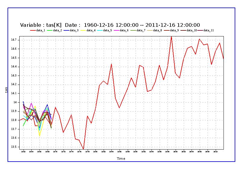
graph¶

Usage


cdo -graph  ifile1 ifile2... ofile 

cdo -graph,device="pdf" ifile1 ifile2... ofile 

cdo -graph,ymin=0.0,ymax=10.0 ifile1 ifile2... ofile 

cdo -graph,stat="TRUE" ifile1 ifile2... ofile 

cdo -graph,stat="TRUE",sigma=6.0 ifile1 ifile2... ofile 

cdo -graph,obsv="TRUE" obsvfile ifile1 ifile2... ofile 

cdo -graph,ymin=0.0,ymax=10.0,stat="TRUE",sigma=6.0,obsv="TRUE" obsvfile ifile1 ifile2... ofile

device	Output File format can be "PS","EPS","PDF","PNG","GIF","JPEG","SVG","KML" . Default output format is "PS"
ymin	Minimum value of the y-axis data
ymax	Maximum value of the y-axis data
stat	"TRUE" or "FALSE" , to switch on the mean computation. Default is "FALSE". Will be overridden to "FALSE" if input files have unequal number of time steps or different start/end times.
sigma	Standard deviation value for generating shaded back ground around the mean value.To be used in conjunction with 'stat="TRUE"'
obsv	To indicate if the input files have an observation data, by setting to "TRUE".Default value is "FALSE". The observation data should be the first file in the input file list. The observation data is always plotted in black colour.

Sample Images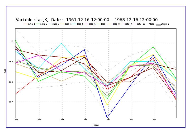

contour¶

Usage


cdo -contour  ifile ofile

cdo -contour,device="pdf"  ifile ofile

cdo -contour,min=0.0,max=10.0  ifile ofile

cdo -contour,count=20  ifile ofile

cdo -contour,interval=5.0  ifile ofile

cdo -contour,list="5.0;7.0;10.0"  ifile ofile

cdo -contour,colour="green" ifile ofile

cdo -contour,RGB="TRUE",colour="RGB(0.0;1.0;1.0)" ifile ofile

cdo -contour,thickness=5.0  ifile ofile

cdo -contour,style="DASH" ifile ofile

cdo -contour,colour="RGB(100.0;100.0;100.0)" ifile ofile

cdo -contour,device=gif_animation,step_freq = 20 ifile ofile

cdo -contour,min=0.0,max=10.0,count=20,RGB="TRUE",colour="RGB(0.0;1.0;0.0)",thickness=10.0,style="DASH" ifile ofile

device	Output File format can be "PS","EPS","PDF","PNG","GIF","GIF_ANIMATION","JPEG","SVG","KML" . Default output format is "PS".
min	Minimum value of the data for generating the contour plot
max	Maximum value of the data for generating the contour plot
count	Number of contour levels
interval	Interval in data units between two bands lines
list	List of levels to be plotted
RGB	To indicate, if the input colour is in RGB format
colour	Colour for drawng the contours, can be either standard name or in RGB format
thickness	Thickness of the contour line
style	Line Style can be "SOLID","DASH","DOT","CHAIN_DASH","CHAIN_DOT"
step_freq	Frequency of time steps to be considered for making the animation( device = gif_animation). Default value is "1" (all time steps). Will be ignored if input file has multiple variables
file_split	To split the output file for each variable, if input has multiple variables.Values can be "TRUE" or "FALSE". Default value is "FALSE". Valid only for "PS" format.

shaded¶

Usage


cdo -shaded ifile ofile

cdo -shaded,device="pdf"  ifile ofile

cdo -shaded,min=0.0,max=10.0  ifile ofile

cdo -shaded,count=20  ifile ofile

cdo -shaded,interval=5.0  ifile ofile

cdo -shaded,list="5.0;7.0;10.0" ifile ofile

cdo -shaded,colour_min="green",colour_max="blue",colour_triad="CW"  ifile ofile

cdo -shaded,RGB="TRUE",colour_min="RGB(0.0;0.0;1.0)",colour_max="RGB(1.0;0.0;0.0)",colour_triad="CW" ifile ofile

cdo -shaded,RGB="TRUE",colour_min="red",colour_max="blue" ifile ofile

cdo -shaded,colour_min="RGB(0.0;0.0;1.0)",colour_max="RGB(1.0;0.0;0.0)" ifile ofile

cdo -shaded,count=5,colourtable="table.txt" ifile ofile

cdo -shaded,min=-10.0,max=10.0,count=20,RGB="TRUE",colour_min="RGB(0.0;0.0;1.0)",colour_max="RGB(1.0;0.0;0.0)" ifile ofile

device	Output File format can be "PS","EPS","PDF","PNG","GIF","GIF_ANIMATION","JPEG","SVG","KML" . Default output format is "PS"
min	Minimum value of the data for generating the grid fill plot
max	Maximum value of the data for generating the grid fill plot
count	Number of colour bands
interval	Interval in data units between two bands lines
list	List of levels to be plotted
RGB	To indicate, if the input colour (i.e,colour_min, colour_max) is in RGB format
colour_min	Colour for the Minimum colour band,can be either standard name or in RGB format
colour_max	Colour for the Minimum colour band,can be either standard name or in RGB format
colour_triad	Direction of colour sequencing for shading "CW" or "ACW" , to denote "clockwise" and "anticlockwise" respectively. To be used in conjunction with "colour_min", "colour_max" options. Default is "anticlockwise"
colour_table	File with user specified colours with the format as ( example file for 6 colours in RGB format )(can be either standard name or in RGB format.)
step_freq	Frequency of time steps to be considered for making the animation( device = gif_animation). Default value is "1" (all time steps). Will be ignored if input file has multiple variables
file_split	To split the output file for each variable, if input has multiple variables.Values can be "TRUE" or "FALSE". Default value is "FALSE". Valid only for "PS" format.

6
RGB(0.0;0.0;1.0)
RGB(0.0;0.0;0.5)
RGB(0.0;0.5;0.5)
RGB(0.0;1.0;0.0)
RGB(0.5;0.5;0.0)
RGB(1.0;0.0;0.0)

grfill¶

Usage


cdo -grfill  ifile ofile

cdo -grfill,device="pdf"  ifile ofile

cdo -grfill,min=0.0,max=10.0  ifile ofile

cdo -grfill,count=20   ifile ofile

cdo -grfill,interval=5.0   ifile ofile

cdo -grfill,list="5.0;7.0;10.0"   ifile ofile

cdo -grfill,resolution=15.0   ifile ofile

cdo -grfill,colour_min="green",colour_max="blue"   ifile ofile

cdo -grfill,colour_min="green",colour_max="blue",colour_triad="ACW"   ifile ofile

cdo -grfill,RGB="TRUE",colour_min="RGB(0.0;1.0;0.0)",colour_max="RGB(0.0;0.0;1.0)" ifile ofile

cdo -grfill,RGB="TRUE",colourtable="table.dat" ifile ofile

cdo -grfill,min=-10.0,max=10.0,count=20,RGB="TRUE",colour_min="RGB(0.0;0.0;1.0)",colour_max="RGB(1.0;0.0;0.0)",resolution=15.0 ifile ofile

device	Output File format can be "PS","EPS","PDF","PNG","GIF","GIF_ANIMATION","JPEG","SVG","KML" . Default output format is "PS"
min	Minimum value of the data for generating the grid fill plot
max	Maximum value of the data for generating the grid fill plot
count	Number of colour bands
interval	Interval in data units between two bands lines
list	List of levels to be plotted
RGB	To indicate, if the input colour (i.e,colour_min, colour_max) is in RGB format
colour_min	Colour for the Minimum colour band,can be either standard name or in RGB format
colour_max	Colour for the Minimum colour band,can be either standard name or in RGB format
colour_triad	Direction of colour sequencing for shading "CW" or "ACW" , to denote "clockwise" and "anticlockwise" respectively. To be used in conjunction with "colour_min", "colour_max" options. Default is "anticlockwise"
resolution	Number of cells per cm for CELL shading
colour_table	File with user specified colours with the format as ( example file for 6 colours in RGB format )( can be either standard name or in RGB format )
step_freq	Frequency of time steps to be considered for making the animation( device = gif_animation). Default value is "1" (all time steps). Will be ignored if input file has multiple variables
file_split	To split the output file for each variable, if input has multiple variables.Values can be "TRUE" or "FALSE". Default value is "FALSE". Valid only for "PS" format.

6
RGB(0.0;0.0;1.0)
RGB(0.0;0.0;0.5)
RGB(0.0;0.5;0.5)
RGB(0.0;1.0;0.0)
RGB(0.5;0.5;0.0)
RGB(1.0;0.0;0.0)

vector¶

Usage


cdo -vector  ifile ofile

cdo -vector,device="pdf" ifile ofile

cdo -vector,thin_fac=5.0  ifile ofile

cdo -vector,unit_vec=55.0  ifile ofile

cdo -vector,thin_fac=5.0,unit_vec=55.0  ifile ofile

Important: the vector variables have to be 'u' and 'v'. To change the variable names e.g. from 'u10' and 'v10' use -chname,u10,u,v10,v before creating the vector plot like:

cdo vector,device="pdf",thin_fac=2.0,unit_vec=20.0 -seltimestep,1 -chname,u10,u,v10,v -selvar,u10,v10 <infile> <outfile>

device	Output File format can be "PS","EPS","PDF","PNG","GIF","GIF_ANIMATION","JPEG","SVG","KML" . Default output format is "PS"
thin_fac	Controls the actual number of wind arrows or flags plotted. See Magics++ library for explanation
unit_vec	Wind speed in m/s represented by a unit vector ( 1.0 cm )
step_freq	Frequency of time steps to be considered for making the animation( device = gif_animation). Default value is "1" (all time steps). Will be ignored if input file has multiple variables

NOTE: The valid standard name strings for "colour" are

"red", "green", "blue", "yellow", "cyan", "magenta", "black", "avocado",
"beige", "brick", "brown", "burgundy","charcoal", "chestnut", "coral", "cream",
"evergreen", "gold", "grey", "khaki", "kellygreen", "lavender",
"mustard", "navy", "ochre", "olive","peach", "pink", "rose", "rust", "sky",
"tan", "tangerine","turquoise","violet", "reddishpurple",
"purplered", "purplishred","orangishred", "redorange", "reddishorange",
"orange", "yellowishorange","orangeyellow", "orangishyellow",
"greenishyellow", "yellowgreen","yellowishgreen", "bluishgreen",
"bluegreen", "greenishblue","purplishblue", "bluepurple",
"bluishpurple", "purple", "white"

Tips and tricks for high resolution data¶

High resolution data sets have a couple of extra properties, which make them a little harder to work with

Input files are usually huge - quite obvious, I know, but it's good to keep that in mind if things take much longer than usual. Computing a global mean value of 80 million grid points just takes longer than on 80000, so be patient!
The large file size implies an even larger influence of IO on the total performance. Early data reduction/selection is a must as well as avoidance of temporary file creation. It can be worth checking the actual reading/writing performance of your system in order to estimate which worklow works best: write interim results of mediate or large size and base next computations in them or work with complex CDO calls to write down very small result files.
File size can be misleading though: NetCDF and GRIB2 have very effective compression algorisms built-in (zip-compressed nc4, aec/szip compressed grb2). The downside is that in both cases decompression is slow. Especially with large horizontal fields the time for decompressing supersedes the saved read-in time compared to uncompressed data. These compressions are essentially made for saving storage space, but not for extensive work with the data.
Due to the fact, that the coordinates themselves are big fields, they are usually not attached to high resolution data files to save disk space. Hence they have to be attached on-the-fly for any of operation that needs them, e.g. sellonlatbox, fldmean, ...
Don't hesitate to selection regions on unstructured grids with the usual sellonlatbox operator: Originally designed for regular grids, it now (cdo-1.9.5) uses very fast search algorithms for any kind of grids.
Some words on interpolation: Consider pre-computing interpolations weight even if you have multiple regions of interest. The weight generation itself is OpenMP-parallelized and scales well, the application of these weight be parallelized using multiple processes

Lets go through some examples step by step

remapping

cdo -P 12 -genycon,${out_dir}/0.10_grid.nc \
          -setgrid,${tmp_dir}/FV3-3.25km/gridspec.nc:2 \
          -collgrid,gridtype=unstructured ${fv3_dir}/FV3-3.25km/2016080100/lhflx_15min.tile?.nc  \
           ${tmp_dir}/FV3-3.25km/fv3_weights_to_0.10deg.nc
cdo -P 12 -remap,${out_dir}/0.10_grid.nc,${tmp_dir}/FV3-3.25km/fv3_weights_to_0.10deg.nc \
          -setgrid,${tmp_dir}/FV3-3.25km/gridspec.nc:2 
          -collgrid,gridtype=unstructured ${fv3_dir}/2016080100/${var}_15min.tile?.nc \
           ${tmp_dir}/FV3_${var}_1.nc

selection

cdo -s -f nc -copy \
             -sellonlatbox,${lonMin},${lonMax},${latMin},${latMax} \
             -remap,${grid},${weights} \
             -selvar,tp ${inpFile} \
             ${outDir}/tmp_${fileIdx[i]}.nc

any ideas?

cdo -infov -div -fldmean -cat [ -for,1,10 -mulc,-1 -for,1,5 ] -fldmax -topo

CDO option --worker¶

The CDO option "--worker <N>" set the number of workers to asynchronously decode/decompress <N> GRIB records.
This can improve the performance of reading compressed GRIB files. The speedup and memory usage depends on
the size of the grid, the number of records per timestep and the used CDO operators.
The option --worker is available since CDO release 1.9.7.

Here is an example of "cdo info" on an AEC compressed GRIB2 file containing ICON R2B9 data with one 3D variable
on 77 levels and 8 timesteps:

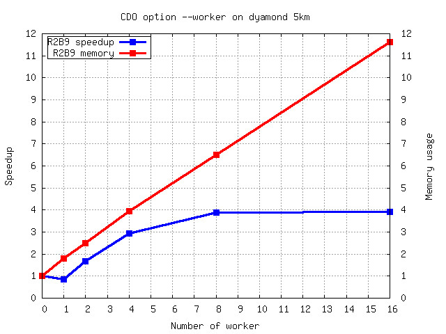
The speedup with 4 workers is 3 and it doesn't scale with more than 8 workers.

The I/O is synchronized after each timestep. That means the worker pipeline needs to be flushed at the end
of a timestep and refilled at the beginning of the next timestep. Therefor the number of records per timestep
must be much higher than the number of worker in order to improve the performance.

Be careful when using any selection operator in combination with other CDO operators.
This will start all worker with decompressing the next records also if they are not selected.
This could slow down the performance of the processing.

Files (4)

ifs2icon_skel.rb (1.14 KB) ifs2icon_skel.rb		Ralf Mueller, 2012-09-12 10:24
teststat.jpg (70.1 KB) teststat.jpg		Kameswarrao Modali, 2012-10-16 17:17
testall.jpg (74.1 KB) testall.jpg		Kameswarrao Modali, 2012-10-16 17:17
cdo_worker.jpg (83.2 KB) cdo_worker.jpg		Uwe Schulzweida, 2019-06-12 14:26

Project

General

Profile

CDO

Wiki

Tutorial¶

Introduction¶

Basic Usage¶

Make variable modifications¶

Combining Operators¶

The expr Operator¶

The select and delete Operator¶

Missing values¶

Autocompletion¶

Using CDO from other languages¶

High performance processing¶

Masking¶

Interpolation¶

Horizontal fields¶

Vertical fields¶

Time interpolation¶

Plotting¶

graph¶

contour¶

shaded¶

grfill¶

vector¶

Tips and tricks for high resolution data¶

CDO option --worker¶